In this part 1, we will look at getting a better understanding of a stochastic process, in the next one we will look at some practical implementations to build on this understanding to solve some real-world problems.
What is a Stochastic Process
Wikipedia defines a stochastic process as a mathematical object that is defined by a family of random variables.
A better way to look at it would be
It is a collection of random “events”, each happening with either fixed or varying probabilities, over a given time
where events can be a single experiment or a cluster of them, for example: Tossing a coin is an event, as we will have a measurable outcome out of the same.
In fact, a good example of a stochastic process can be coin tosses happening over a period of time, say we do 100 coin tosses in 100 minutes. The process of these coin tosses will be a discrete stochastic process, where events will be individual coin tosses.
In this particular implementation, we will try and understand this simple stochastic process or Random walk and in the next one, we will see how they are used to model things like stock movements, particle behavior in solutions, etc.
Creating a discrete stochastic process
Let’s take into consideration the mathematics of a simple experiment, the rules of the experiment are as follows:
There are two players, one X, and the other Y
- Each takes a turn to flip a fair coin.
- Before flipping this coin, each one bets one dollar(only because it sounds cool) on the outcome.
- If we get heads X wins all the money (1 dollar of Y and takes back his own dollar as well), similarly, if we get tails Y takes all the money.
- The game will go on until X wins 50 dollars or lose 50 dollars
Now since we know that the “events” are simple fair coin tosses, we can easily deduce that the probability of each event to be heads or tails is
½ or 0.5
We also know that this process is done over a certain period of time, let us take the time to be presented by variable t.
We further know from our definition that a stochastic process can be represented as a function of time, and each time step is independent of all the previous occurrences (each coin toss is independent and is not influenced by the results of the previous results). Therefore we can represent this stochastic process as:
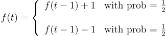
Understanding the formula
Let’s dissect this formula real quick.
At any given time after starting initially at zero, we will be in any one of the three states:
We are back at 0, meaning, x has won as many times as y.
We can be at a point above 0, meaning x has won more times than y.
We can be at a point below 0, meaning x has lost more times than y.
Now at any given time t, we will be in either one of these stages, represented by the part f(t - 1 ) meaning all the events that have happened until the previous time step, now although our state depends on the previous states(meaning if we are above or below 0), what happens at time t within the event is independent. (The coin toss is still fair with probability ½ ).
In light of the same we can either win 1 dollar meaning we can have f ( t - 1 ) + 1 (with chances of the same happening being ½ ) or we can loose 1 dollar meaning we can have f ( t - 1 ) - 1 (with chances of the same happening being ½ )
Simulating the same with python
The same is understood better by this simple simulation of this process where we present the earnings/losses of x when playing this particular game.
Now doesn’t this thing looks like something? for those of you who follow, these moves exactly look similar to a stock, so can we use stochastic process to map the outcome of stocks? Well, stay tuned to look for answers in the next one in this series.
The code to get the simulation running is accessible here
**The title image is from coursera