I came across Bayesian theorem a lot early in my education carrier, much like Thomas Bayes himself, I was not able to grasp the importance of this masterpiece. Additionally, much like most of the concepts at the time I just jumped over the understanding of the same and was mostly focused on solving some predefined pattern questions and never bothered to figure out how the theorem can actually be put to use in the real-world implementations. Now when I look back it was not a very wise decision to make, as almost all of the risk management strategies in my automated trading algorithms were impossible without Bayes and his work, particularly the Bayes theorem.
Once I did realize my mistake I spent good 2 weeks on trying to get the hold of it, watching countless videos, going through a number of blogs, and posts around the same. No significant headway was being made, as I was always able to sort of get the idea and remember the formula maybe think of the use case that was explained in the blog or the video, but the true understanding was missing, the level of comfort I intended to have with it was just not there, which was very frustrating to say the very least.
The worst part about not being able to understand something properly is that people who do understand always make it look so trivial so easy, one feels like probably I am dumb and I am just MESSING never going to be good enough to be able to understand anything and should just quit. Well thankfully I didn’t and now I think I have a pretty good understanding of the same. I will outline how I understood this classic and maybe that is helpful to someone who is going through the same phase.
If I were, to sum up, a learning lesson for logical thinking that I had taken away from Bayesian is
“The new or current evidence should not cause us to discard the old beliefs completely but to merely update the same with the new information coming in”
The big example
I was most intrigued by the Conjunction fallacy, it is an example of irrational[?] behavior in an experiment by renowned Nobel Prize winner Daniel Kahneman, I will borrow explanation of the setup from wikipedia, the link to the complete explanation is accessible here. I have taken the liberty to use a simpler version for the sake of understanding but we are able to get home with understanding just as well.
The most often-cited example of this fallacy originated with Amos Tversky and Daniel Kahneman. Although the description and person depicted are fictitious, Amos Tversky secretary at Stanford was named Linda Covington, and he named the famous character in the puzzle after her.

Linda is 31 years old, single, outspoken, and very bright. She majored in philosophy. As a student, she was deeply concerned with issues of discrimination and social justice, and also participated in anti-nuclear demonstrations.

Which is more probable?

1. Linda is a bank teller or a farmer ?

We will further assume that we have access to results of focus groups to pin point traits for farmers and bank tellers related to the evidence.
Bayesian Approach
Now this is an interesting problem to solve, but to make a logical conclusion we need to draw from our previous understanding of the the Bayes Theorem, recall that we had prophesied that new evidence or new data should not create new beliefs but should update our existing beliefs.
Let us review this problem now in light of Bayes theorem so we are able to make an appropriate[?] approximation of the outcomes. For the sake of understanding we will assume that the we are going to select bank teller in the above experiment and are only interested in validating and rejecting this hypothesis. (Since if we validate or reject this hypothesis we will inventively be making a conclusion, i.e. if Linda is not a bank teller she will be a farmer)
In this particular case the evidence for us will be the traits for Linda, where we have information about the age and views on certain socio-political issues.
Before that lets get few jargons out of the way first so we are able to focus on the fun stuff:
Prior
It is the information we have before the evidence was introduced, in our librarian example it will be the proportion of bank tellers to the number of farmers. We will represent this information with P(H) which in our case is 10/100 (Meaning we have 10 bank teller for every 100 sample we take of bank tellers and farmers). Therefore
P(H) = 0.1
Similarly the probability when the hypothesis is not correct in any given sample (It is represented with a “~” which denotes not)
P(~H) = 0.9Likelihood
It is the probability of the number of instances in which the hypothesis is true, given the evidence. In probability we usually use symbol “|” to represent given so (E|H) will be read as probability of E given that H has happened. In our case this will be the information we have for the traits of farmers and bank tellers from a focus group study. Let us assume that the information in the group study puts the proportion of bank tellers with the given traits to be 40%, meaning there is 40% chance that a bank teller has similar traits to Linda, and there are also 10% farmers with traits similar to Linda.
From the above information we can put that the likelihood of the similar events (Bank teller with given traits) being true is given by
P(E|H) = 0.4 {4/10}Similarly we will also need to account for the farmers who have similar traits, which we know are 10%, therefore
P(E|~H) = 0.1 {10/100}
(where P(E|~H) means existence of evidence when the hypothesis is not true )Posterior
It is the final probability we are going to assign to our hypothesis being correct when we have plugged in information about the evidence. It is going to be denoted by P(H|E), meaning probability of H given E(Probability that the hypothesis is true give the evidence)
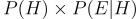
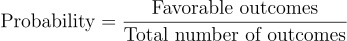
Now having all the details at our disposal we just need to just use a pretty simple mechanism, remember we use to define probability as merely the the ratio of favorable outcomes to total possible outcomes. favorable outcomes in our case are going to be that Linda is a Bank teller and has the given traits, essentially meaning, “Prior x Likelihood”, which is
Similarly the total probability of seeing the evidence in any form will be equal to, probability of seeing the evidence when the hypothesis is correct and probability of seeing the evidence when the hypothesis is incorrect. which is essentially given by

So essentially we have broken down the problem into the simple form of probability where we have to just fill in the formula.Essentially
which as per our discussion corresponds to simply
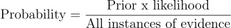
which in turn corresponds to
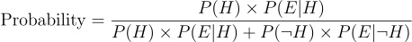
This is nothing but Bayes theorem
Back to example
Summing up and substituting values that we have already attained for the individual components above for our POI Linda we can simply validate the changes of success for our hypothesis to be equal to
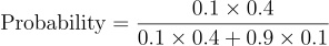
which comes out to be 0.30769230769230776
meaning there are only 30% chances of success if we select Linda to be Bank Teller, therefore its more reasonable to play the odds and select Linda to be a Farmer even when she has more traits common with Bank Tellers, which is synonymous with our initial understanding that new information should only update the old belief or Prior
Also this is the value for Posterior = 0.30769230769230776
** Shared image credits Researchgate